We have just had the definition of a pullback; now in Awodey pages 95 through 100 we’ll see some more about them, and after that we’ll get the more general unifying idea of the limit in pages 100 through 105.

Lemma 5.8 states that a certain commuting diagram is a pullback. The proof is by “diagram chase”, and I can see why - my proof goes along the lines of gesturing several times at various parts of the diagram. Then the corollary takes me a moment to get my head around, but then I turn my head sideways and it pops out of the diagram. If you push the \(h’\) line into the page in Lemma 5.8, and rotate the diagram by ninety degrees, you end up with the diagram of Corollary 5.9; then part 2 of Lemma 5.8 is the corollary.

The operation of pullback is a functor. Given a “base” arrow \(h\), we may define a functor which takes an arrow \(f\) and pulls back along \(f, h\). It seems very plausible, but it takes me a while of staring at the diagrams before it makes sense. In particular, the diagram in the book doesn’t do a good job of splitting up the two statements which are proved: namely that \(h^* 1_X = 1_{X’}\) and \(1_{X’} = 1_{h^* X}\).

The corollary is that \(f^{-1}\) is a functor, which follows because the operation “pull things back along \(f\)” is a functor. Then we get that \(f^{-1}\) descends to the quotient by equivalence. This is all a set of symbols which I barely understand, so I have a break and the go back over the whole thing again.

Pullback is a functor. Fine. Then \(f^{-1}: \text{Sub}(B) \to \text{Sub}(A)\) - which is defined as the pullback of an inclusion and \(f\) - must also be a functor, because it is exactly the operation “take a certain pullback”. The statement that \(M \subseteq N \Rightarrow f^{-1}(M) \subseteq f^{-1}(N)\) is just the statement that “if we apply the pullback by \(f\) and an inclusion, the relation \(\subseteq\) is preserved”, which is true because pullback is a functor. (Recall that \(M \subseteq N\) iff there is \(g: M \to N\) with the triangle \(m: M \to Z, n: N \to Z\) commuting. We’re working throughout with subobjects of the object \(Z\).)

Now we do have \(M \equiv N\) implies \(f^{-1}(M) \equiv f^{-1}(N)\) - recall that \(M \equiv N\) iff both are \(\subseteq\) each other - so \(f^{-1}\) is constant on equivalence classes and so descends to the quotient. That’s a bit clearer now.

Phew, a concrete example is coming up: a pullback in Sets. I draw out the general diagram first, then write in the assumptions we make, and end up with a diagram a lot like the one in the book, except that I’ve labelled the unlabelled arrow “inclusion”.

Ah, I’m starting to get this. The operation “take inverses” is a function which takes one “major” argument \(f: A \to B\), and one “minor” argument \(M\) (from which we extract the corresponding subset-arrow \(m: M \to B\)). The output is the pullback diagram, which may be interpreted as just the pullback object from those two arrows.

Once I’ve realised that the operation “take inverses” is as above, the top of the following page (p99) becomes trivially obvious, although I still have to do some mental work to do the interpretation in terms of substituting a term \(f\) for a variable \(f\) in function \(\phi\). It seems like a very complicated way of saying something very simple.

Then we see the naturality of the isomorphism \(2^A \cong \mathbb{P}(A)\). First, am I convinced we’ve even shown that there is an isomorphism? Certainly each function \(A \to 2\) corresponds (by inverses) to a unique member of \(\mathbb{P}(A)\), while each member of \(\mathbb{P}(A)\) corresponds to a unique member of \(2^A\) given by the characteristic function. Now, does the naturality diagram really commute? Yes, that’s what happened above: \(f^{-1}(V_{\phi}) = V_{\phi f}\).

This section has one final example: reindexing an indexed family of sets. The definition of \(p\) is fine; then we pull it back along \(\alpha\). I need to check that the guessed pullback object is indeed a pullback, for which I need a diagram. The required property eludes me completely until I realise that the topmost arrow of Awodey’s diagram is in fact the identity; then the UMP falls out easily.

Section 5.4 is entitled “limits”, and it promises to unify pretty much everything we’ve already seen. Recall the theorem that if a category has pullbacks and a terminal object if has finite products and equalisers, because we may take the equaliser of the product to obtain a pullback, and we may perform the empty product to obtain a terminal object. Now Awodey proves the converse: constructing the product as a pullback from a terminal object, and constructing the equaliser as a pullback of the identity pair of arrows with the pair \(\langle f, g \rangle\) we want to equalise.

Define a “diagram of type \(\mathbf{J}\) in \(\mathbf{C}\)” in the way you’d hope: since an arrow \(X \to Y\) is thought of as a shape-\(X\) subset of \(Y\), we should consider a shape-\(\mathbf{J}\) “subset” of \(\mathbf{C}\) to be a functor \(\mathbf{J} \to \mathbf{C}\).

Define a cone to the diagram \(D\) as - well, the name is quite suggestive. Fix a base object \(C\) of \(\mathbf{C}\), and then the subcategory of all the arrows \(C \to D_j\) forms a category of shape \(\mathbf{J}\) in \(\mathbf{C}\), all linked to this base \(C\). (Of course, we insist that the arrows of this cone commute with the base object.)

A morphism of cones behaves in the obvious way: send the base point to its new position, and send each arrow to its new arrow. (We keep the \(D_j\) the same, because we need to preserve the diagram; we’re only changing the position of the apex of the cone.)

Finally, the definition of a limit! It’s a terminal object in the category of cones on a given diagram. All cones have exactly one arrow going into this cone (if it exists). The “closest cone to the diagram” idea is a nice one, and I can see how this links with the idea of a universal mapping property. The UMPs we’ve seen up to now are of the form “draw this diagram, and select the closest object that fulfils it” - how neat. This immediately covers the product, pullback and equaliser examples; from the empty diagram, there is precisely one cone for each object (namely “pick a vertex, and have no maps at all”), so the category of cones is just the original category, so the limit is a terminal object.

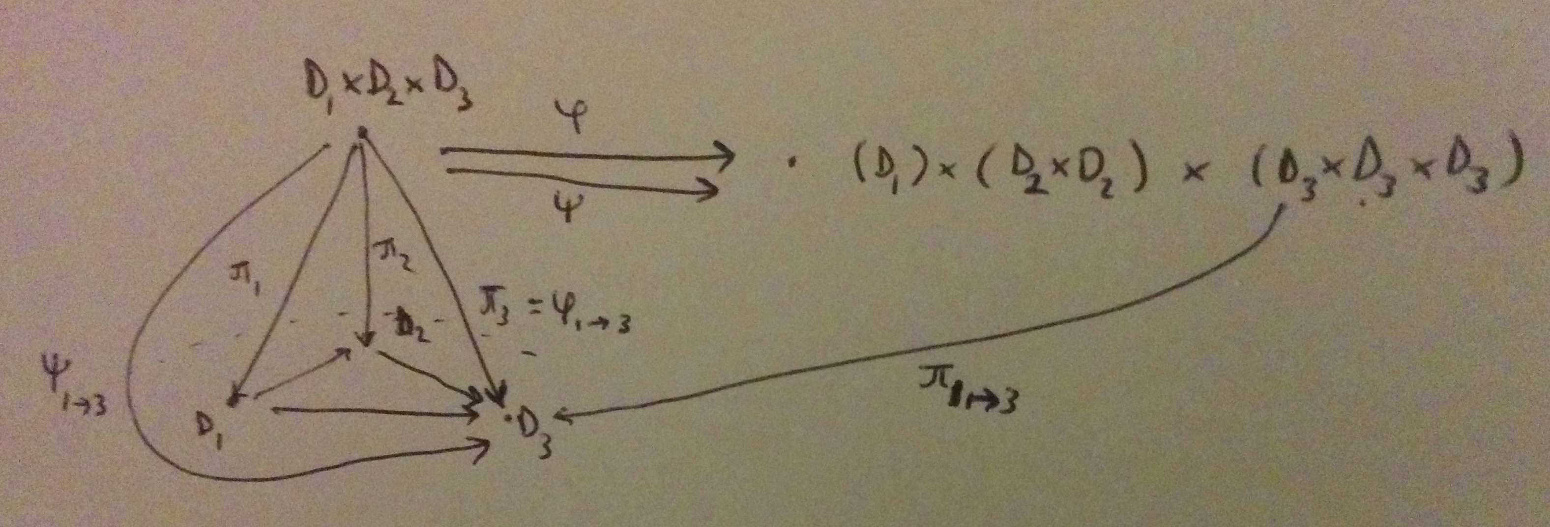
Now, a theorem on an equivalent condition for having all finite limits. If a category has all finite limits, then it trivially has all finite products and equalisers, because they’re limits. Therefore we need to show that if a category has all finite products and equalisers, then we can build any limit. The proof will have to start by fixing some finite category \(\mathbf{J}\) and considering some fixed diagram of shape \(\mathbf{J}\) in \(\mathbf{C}\). Construct the cone category. We’re going to have to manufacture the limit somehow, given that we have finite products and equalisers. At this point I look in the book and it tells me that the first step is to consider the product of all the objects in the diagram. OK, that is a cone-shape - it has the right arrows. Could it be a limit? We’d need that for any other cone \(X\), there was a unique arrow \(X \to \prod D_i\) commuting with the projections. That doesn’t actually hold, though: consider \(D_1, D_2\) as our diagram, and take \(D_1 \times D_2\) as the product. Then \(D_1 \times { \langle x, x \rangle : x \in D_2 }\) doesn’t have a unique arrow into \(D_1 \times D_2\), because we could take either the second or the third projection, so we want to equalise out by such manipulations.

Ugh, I just don’t see how to do this. I’ll have to look at the book again. The construction is quite complicated: we take the product over all the possible arrows (ways to get to) \(D_j\) from any object \(D_i\), and we’ll equalise out the different ways to get to each object. This becomes much clearer from a diagram, where it actually looks like the only possible way to do it: basically list all the different ways to get from A to B, and equalise out by “viewing them all as being the same way”.

Once that’s done, the rest is bookkeeping to check that we’ve actually made a cone, and that the cone is a limit, by showing that “cone” is precisely “thing which satisfies the equaliser diagram”; then the fact that we made a limit falls straight out of the uniqueness part of the UMP.

The final bit on “we didn’t use the finiteness condition” is clear, and the dual bit is clear (though I have not much idea about what a colimit or a cocone is). Presumably we’ll see some examples of colimits later, but I imagine the coequaliser and coproduct are examples.

Summary

This section was really neat. Quite hard to understand - took a lot of time and effort to get the pullbacks idea - but the feeling of unification was great fun. Next up will be “preservation of limits” and colimits, and after that will come some exercises (which I think are sorely needed). Then the next chapter is on another kind of construction which is not a limit, and then the really meaty sections which Awodey has called “higher category theory” and which occupy a large chunk of the Part III introductory category theory course.