In my latest lecture on Markov Chains in Part IB of the Mathematical Tripos, our lecturer showed us a very nice little application of the theorem that “if a discrete-time chain is aperiodic, irreducible and positive-recurrent, then there is an invariant distribution to which the chain tends as time increases”. In particular, let \(X\) be a Markov chain on a state space consisting of “the value of a card revealed from a deck of cards”, where aces count 1 and picture cards count 10. Let \(P\) be randomly chosen from the range \(1 \dots 5\), and let \(X_0 = P\). Proceed as follows: define \(X_n\) as “the value of the \(\sum_{i=0}^{n-1} X_i\)-th card”. Stop when the newest \(X_n\) would be greater than \(52\).

That is, I shuffle a pack of cards, and you select one of the first five at random. I then deal out the rest of the cards in order; you hop through the cards as they are revealed. For instance, if the deck looked like \({5,4,9,10,1,2,6,8,8,3, \dots }\) and you picked \(2\) as your starting value, then your list of numbers would look like \({4, 2,8, \dots }\) (moving forward four cards, then two, then eight, and so on). We keep going until I run out of cards to deal out, at which point I triumphantly announce the value of the card which you last remembered.

How is this done? The point is that we are both walking along the same Markov chain, just from different starting positions. As soon as we both hit the same card, we are locked together for all time, and it is simply a matter of ensuring that we hit the same card at some point. But this is precisely what the quoted theorem tells us: if we go on for long enough, we will fall into the same distribution, and hence will likely hit the same card as each other at some point. I ran some simulations to determine the probability with which we end on the same value. The code is kind of dirty, for which I apologise - it was thrown together quickly, and is written in the write-only Mathematica. We first assume that all picture cards are 10s, and that aces are 1s.

nums = Flatten[{ConstantArray[Range[1, 10], 4], ConstantArray[10, 12]}];

The following function runs one simulation using each of the supplied starting indices, using the given order of cards:

test\[perm\_, startPos\_List] := ({Length[#[[1]]], #[[2]]} &@ NestWhile[{#[[1]\]\[[#[[2\]] + 1 ;;]], #\[[1]\]\[[#[[ 2\]]]]} &, {perm, #}, Length[#[[1]]] #[[2]] &]) & /@ startPos

It is astonishingly illegible. Read it as: “For each starting position supplied: start off with the input permutation and starting position. While the starting position is a valid position of the list (so it is less than or equal to the length of the list), set the starting position to the value of the card at that starting position, and set the list of cards to be everything after that position. Repeat until we’ve run out of cards. Then output the length of the remaining list of cards [and hence, indirectly, the final position we hit], and the last value we remembered.”

The following line of code runs a hundred thousand simulations with a random order of cards each time:

True/(False + True) /. Rule @@@ Tally[ Function[{inputStartPos}, #[[1, 1]] == #[[2, 1]] &@ test[RandomSample[nums, Length@nums], inputStartPos]] /@ RandomChoice[Range[4], {100000, 2}]] // N

Again, it is illegible. Read it as “We’re going to want the proportion of good results to all results, where “good” is defined as follows: call a run “good” if we stopped at the same card at the end. Do that for a hundred thousand different pairs of random starting points less than \(6\), and tally them all up. Give me a numerical answer at the end, not a fraction.” This program output 0.76764 - that is, there is a better-than-three-quarters chance of “winning” in this variant, where we insist that players pick one of the first five cards to start with, and where we don’t care that queens, kings, jacks and tens are all different.

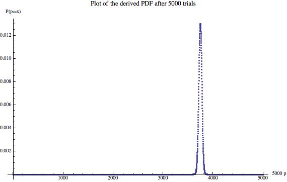
In order to try and be a bit more clever, I used a simple Bayesian update technique to try and get the confidence of the answer. Performing 5000 trials and updating from a prior of “uniformly likely that the required probability is any \(\dfrac{n}{5000}\) for integer \(n\)”, I got the following PDF:

This has mean 0.756297 and standard deviation 0.00606961.

What if we want a different range of starting values? The following table gives the mean and standard deviation of \(p\) for different ranges of allowed starting cards.

N=1: {0.999884, 0.000191799} [the true value is, of course, 1]
N=2: {0.840064, 0.0051822}
N=3: {0.805078, 0.0056006}
N=5: {0.756897, 0.00606454}
N=10: {0.69912, 0.00648421}

How about if we make 10s different from picture cards? Let’s make jacks 11, queens 12 and kings 13:

N=2: {0.834066, 0.00525959}
N=5: {0.716913, 0.0063691}
N=10: {0.673331, 0.0066306}

So your odds of winning are still pretty good, even if we insist that all cards are different (ignoring suit).